Q-Learning

Q-Learning is a value based reinforcement algorithm. The idea is that we create a Q-Table which has all the states represented as rows of Q-table and actions as columns. Then for each state we would select an action which has maximum value (q-value). This means that we do not change/implement a policy that our agent will follow, instead we improve our Q-Table to always choose the best possible action. Lets take an example of Frozen Lake game. The environment is as shown in following image.

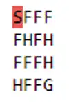
S : Starting point, safe
F : Frozen block, safe
H : Hole, not safe
G : Goal, Our destination

The objective is to determine the shortest possible path to the destination without falling in the hole. The episode ends when you reach the goal or fall in a hole. A reward of 1 is received if you reach the goal and 0 otherwise. In this case, our Q-Table has 16 states and 4 actions (left, right, up, down). Now the question is how do we calculate the q-values to fill the Q-Table? This is where Q-Learning comes into picture.

Given a state and action taken, the Q-function returns an expected discounted (γ = discount factor) future reward of that action for given state. This function is estimated using Q-learning, which updates Q(s,a) using bellman equation.

Q-function

Q(s_t, a_t) = E[R_t+1 + γR_t+2 + γ²R_t+3 + …|s_t, a_t]

Bellman Equation

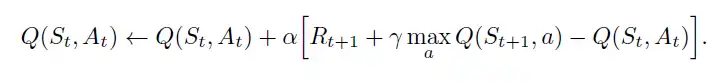
Q(S_t, A_t) = Q value for action taken a in state s at time t.
alpha = learning rate of our algorithm.
R_t+1 = Reward received at time t+1 for action taken in previous state.

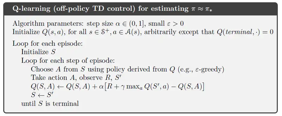
Q-Learning Algorithm

Let’s continue with the Frozen Lake game to understand this algorithm.

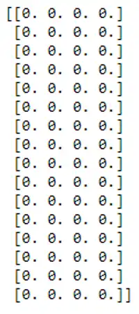
1. Initialize the Q-table to random values. We initialize our Q-table which has 16 rows and 4 columns with zeros.

2. Choose and take action. We chose action (a) for state (s) which has maximum q-value. But initially all the values are zero, this is where the exploration and exploitation strategy comes into play. We use a strategy called epsilon-greedy strategy.
   In this we set the initial value of epsilon to 1 and gradually decrease the value to 0 with time. We draw a random number from a uniform distribution between 0 and 1. If this number is less than the epislon we take a random action. The idea behind this is that, initially as the agent doesn’t know anything about the environment, we take random action i.e we let the agent explore the environment. As agent explores the world, the epsilon value decreases and the agent starts exploiting. Eventually agent becomes confident in estimating the q-values.

3. Evaluate the action taken. After taking action at each time step, we receive a reward. We then use this reward to update our Q-table using the bellman equation.

4. Repeat. We repeat this process again and again untill the learning is stopped.

Check this Jupyter Notebook here for complete python code to solve the Frozen Lake problem using Q-Learning.

(Source: Richard Sutton and Andrew Barto, Reinforcement learning Second Edition 2018)

We can see that when we have limited states, Q-table can be efficient. But what happens when we have lots and lots of states? For example you are playing ‘Ping-Pong’, there can be infinite states…then how do we make Q-Table for such cases? The answer is Deep Q-Learning. In the next article we will learn more about Deep Q-Learning and solve a Cart & Pole problem.