Inventory Optimization: MDP vs RL

Inventory Optimization is a task of maximizing revenue by taking into account the capital investment, warehouse capacity, supply and demand of stock, leadtime and backordering of stocks. This problem has been well researched and is usually presented in form of a Markov Decision Process (MDP). The (s, S) policy is proved to be a optimal solution for such problems.[s: Reorder stock level, S: Target stock level].

Markov Decision Process (MDP) provide a framework to model decision making process where outcomes are partly random and partly under the control of decision maker. The learner or decision maker is called an agent. The agent interacts with the environment which comprises of everything except the agent.

The process flow in a MDP is as follows:

1. We get the current state from the environment
2. Agent takes action from all possible actions for the given state
3. Environment reacts to the action taken by agent and present the reward and next state
4. We modify the agents policy based on the rewards received
5. Agent again acts for the new state using the modified policy

This process continues until the task is accomplished.

Inventory Optimization with MDP

Let’s try to understand how to model inventory optimization problem into MDP.

(Source: Andrew Schaefer, EWO Seminar PPT, Oct 2006)

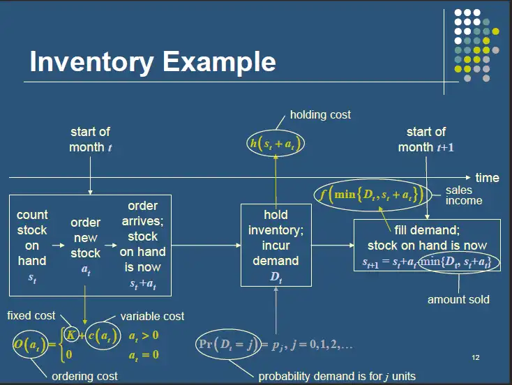
In terms of MDP,

• The states are amount of stock available on hand at start of each time period. Let’s assume the max inventory of our warehouse is M, then all the possible state values can be S_t = 0,1,2,3….M

• The actions are amount of stock that can be ordered at each time period. The possible values for action can be a_t = 0,1,2,3…..M-s_t

• The rewards are expected net income for taking an action in a state. For inventory problem we have 3 costs associated to it as shown above. - Ordering cost - Holding cost - Revenue generated after meeting the customer demand Thus,

  total reward = Expected revenue - order cost - holding cost
  

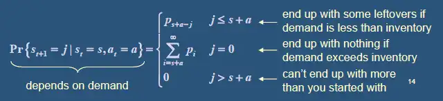
• Transition probabilites govern how the state changes as the actions are taken over time.

(This transition probabilities are for a case where backorders are not accounted for)

The obejective is How much stock should be ordered at each time period such that my expected profits are maximized over time. To solve this problem we make few assumptions:

1. Maximum allowable inventory is M and units can be backordered if sufficient stock is not available to met the customer demand.
2. Demand is random with uniform probability distribution and the values can be 1,2,3,4….M
3. The inventory (state) is counted at the beginning of each time period and a decision is then made to raise the stocks to M.
4. The ordered stock does not have any leadtime and are delivered instanteneously.
5. Customer demand is met at the end of each time period.

With above assumptions, we use (s, S) policy to determine the amount of stock to reorder. In other words, we the stock falls below s, we order the amount such that the inventory is filled up to S.

Let’s take an example:

We have maximum inventory size of 100 units, reorder level (s) is 40 units, restock level (S) = 100, it is (40, 100) policy. We haven’t found the best policy here, which can be found out using value iteration and policy iteration methods. Order cost is 2 per unit, holding cost is 1 per unit, penalty for backorder is 2 per unit, revenue generated is 8 per unit. Check this notebook for complete code.

The average cost per episode with 100 timesteps is 180. The following diagram shows the state vs timestep. Notice, the state value doesn’t go back to 100 in next state as mentioned in our policy, this is because the demand is met at the end of the time period which is subtracted.

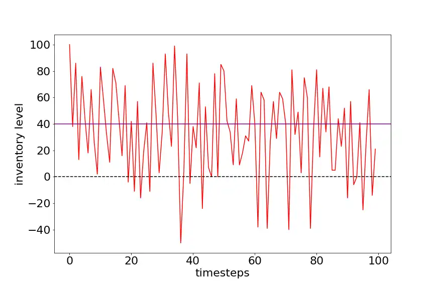
Let’s use this as a baseline to test our model trained using Reinforcement Learning for Inventory Optimization.

Inventory Optimization with Reinforcement Learning

The limitations of MDP is that as the problem size increases, i.e. increase in state and action size, it becomes coputationally difficult to solve the MDPs. Also for each state and action pair we need transition probability which may not be available in real world problem.

Using reinforcement learning removes the need of transition probabilities, and function approximators like neural networks can be used to model enormous state and action space. It is also easier to implement than MDPs.

We create two model types ‘withdemand’ and ’nodemand’. In model type withdemand, the agent is provided with the values of current demand along with current state values to predict the action. Whereas in model type nodemand, the current demand is not disclosed to the agent and the predictions are made based on only current state values. For both model type other information remains the same as defined in MDP. Please check this notebook for full code.

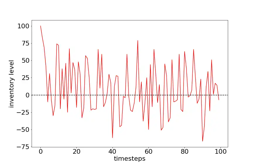
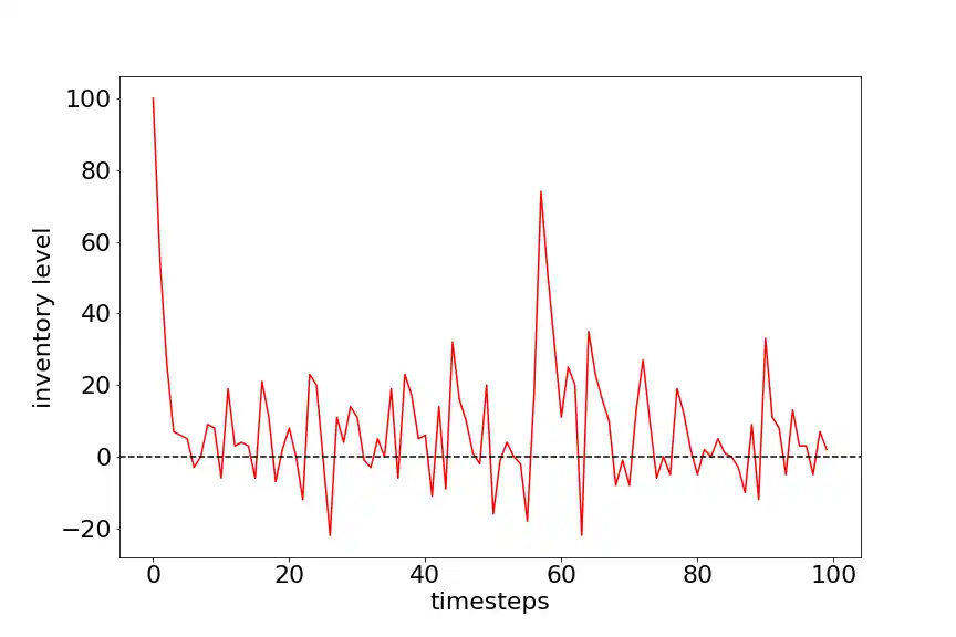
Following plot shows Inventory level vs Timestep for nodemand model type. After training the agent for 500 episodes with 100 timestes each, the average cost per episode with 100 timesteps is 180. From the plot we can see that agent is struggling to keep the backorders and state value to minimum as the demand is unknown.

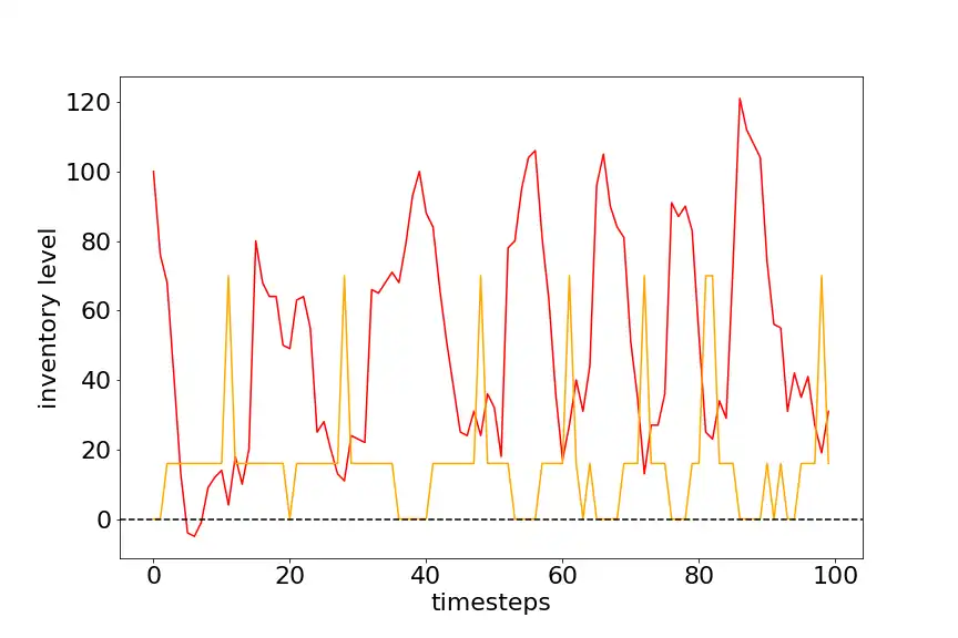
Following graph shows Inventory level vs Timestep for withdemand model type. After training the agent for 500 episodes with 100 timestes each, the average cost per episode with 100 timesteps is 280. The agent is trying to keep the state value close to zero to keep the holding cost to minimum and hence maximizing the rewards.

These models were sucessful in increasing the average profits over a period of time compared to MDP.

Introducing lead time for delivery of stock

Let’s up the game by adding leadtime to the above problem. Assume that there is a lead time of 3 time periods, i.e the action taken at time period t will reach the warehouse at time period t+3. The demand is random with uniform distribution but, it limited to maximum quantity of 30 unit at each time period. In such cases the maximum value of inventory can exceed the value M, thus they are usually modeled as infinite warehouse capacity, i.e there is no upper limit to stocks that can be stored in a warehouse. Although it doesn’t sound correct, but when we train our agent, the agent realizes that keeping excess stocks reduces his profits and thus will try to keep the stock on hand to minimum.

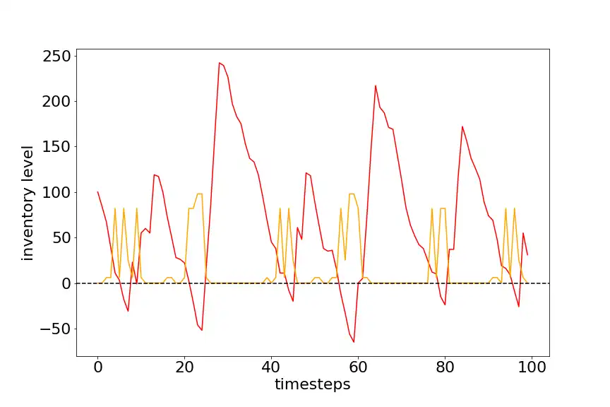
Following graph shows Current state vs Timeperiod for an agent trained for 300 episodes with 500 timesteps each. The current state and demand are given as input to agent to predict the action. The average profit per episode is 30. This is very low as compared to previous solutions, this is because of two main reasons. One, the demand is random and second the agent doesn’t know that there is a lead time of 3 units for the actions taken. Hence, it becomes very difficult to predict the actions so that holding costs are minimized to maximize the profits. The red line indicates the stocks on hand and orange line indicates the action taken (stock ordered) at time period t.

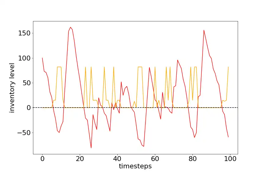
The following graph if for the same agent trained for 400 episodes with 500 timesteps each. It looks like the agent here is trying to keep the order cost to minimum and is therefore ordering large quantities of stock, thus ends up with high on-hand inventory.

The following graph if for the same agent trained for 500 episodes with 500 timesteps each. It is visible that agent has realized it is keep a large stock on hand and thus tries to reduce it. The maximum stock on-hand dropped from 250 to 150, which show that agent partially successful in reducing the on-hand inventory. But now many of the orders are getting backlogged.

There are lots of areas to improve the results further, like giving the stocks in transit as input to our agent along with the current state and demand, testing different hyperparameters for neural net used in our agent, training the agent for longer duration. Complete code can be found here This is just a small example of how reinforcement learning can be used to optimize inventory and maximize the profits in real world.