Graph Neural Networks for Outfit prediction - Part 2

---

Building Your Heterogeneous Graph: From Raw Data to PyTorch Geometric

In our previous post, we explored how to build a Heterogeneous Graph Neural Network (GNN) using PyTorch Geometric. But where does that HeteroData object come from? Today, we’ll dive into the data engineering side of GNNs: how to transform raw tabular data into a graph structure ready for deep learning.

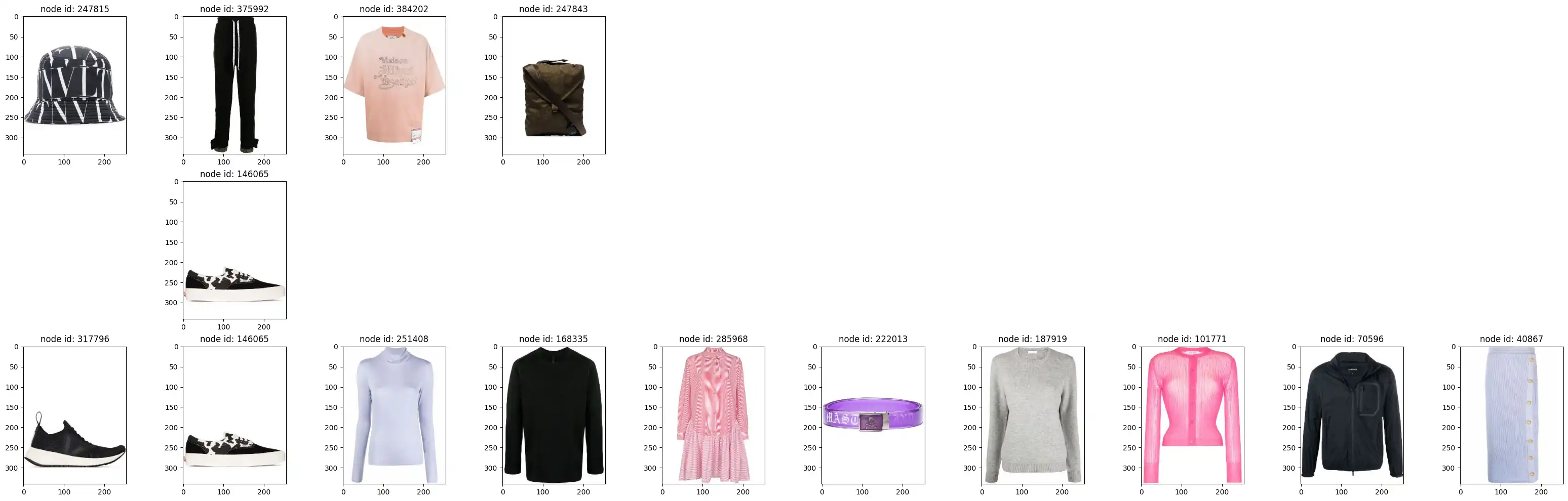
The data used in this tutorial is sourced from the Polyvore Dataset (Maryland Polyvore), which provides high-quality curated outfits and product metadata for fashion research. For more information, visit the official GitHub repository.

Defining the Graph Structure

Our graph represents relationships between products and their metadata. We use two node types and two types of undirected edges:

1. Node Types

• Product: The core entities in our graph. Each product is assigned a unique product_node_id. Features for these nodes are typically derived from text embeddings of descriptions.
• Category: Metadata nodes that help group products. Each unique category gets its own cat_node_id.

2. Edge Types (Undirected)

• Product-Product (product_outfit): Connects two products if they appear together in the same curated outfit. This captures item-item compatibility.
• Product-Category (cat_prod_link): Connects a product to its corresponding category, allowing the model to learn category-level preferences.

In PyTorch Geometric (PyG), nodes are indexed from $0$ to $N-1$. We first create mappings from our original IDs (e.g., SKU strings) to these integer indices.

Step 1: Preparing Nodes

import pandas as pd

# Load raw product data
prod_df = pd.read_parquet('data/products.parquet').reset_index()
# The index becomes our 'product_node_id'
prod_df = prod_df.rename(columns={"index": 'product_node_id'})

# Create a mapping dictionary for later use
p_nodeid_map = prod_df.set_index('product_id')['product_node_id'].to_dict()

# Create category nodes
prod_cat_df = prod_df[['product_category']].drop_duplicates().reset_index(drop=True).reset_index()
prod_cat_df.columns = ['cat_node_id', 'product_category']
cat_nodeid_map = prod_cat_df.set_index('product_category')['cat_node_id'].to_dict()

Step 2: Generating Pre-trained Text Embeddings

A graph structure is only half the story; we also need rich initial features for our nodes. For products, we use Marqo’s E-commerce Embeddings (marqo-ecommerce-embeddings-L).

Why this model?

Standard models like BERT or CLIP are trained on general web text or image-caption pairs. Marqo’s model is fine-tuned specifically for e-commerce, making it significantly better at understanding product attributes, brands, and the nuance of fashion descriptions.

Prompt Engineering for Features

We don’t just embed the description. We construct a rich descriptive string that combines gender, brand, family, category, and highlights:

ptext = (f"This is a {prd_gender} {brand} {family} product and belongs to {category} category, "
         f"{sub_cat_text} sub category. It is a {main_color} color and made of {materials}. "
         f"Highlights: {highlights}. Description: {text}")

Using OpenCLIP, we generate 1024-dimensional embeddings for each product:

import open_clip

model_name = 'hf-hub:Marqo/marqo-ecommerce-embeddings-L'
model, _, preprocessor = open_clip.create_model_and_transforms(model_name)
tokenizer = open_clip.get_tokenizer(model_name)

# Generate features
text_tokens = tokenizer([ptext])
text_features = model.encode_text(text_tokens.to(device), normalize=True)

Step 3: Creating the Edge Indices

Edges are represented as a “COO” format (two rows: source indices and destination indices).

Product to Category Edges

We merge our products with the category IDs we just created.

cat_prod_edge_df = prod_df[['product_category', 'product_node_id']].merge(prod_cat_df, on='product_category')

Product to Product (Outfit) Edges

Outfits are lists of products. We use itertools.combinations to create a link between every pair of products in an outfit.

import itertools

# train_outfits_df contains a column 'products' which is a list of product_ids
outfits_edges_df = train_outfits_df['products'].apply(lambda x: list(itertools.combinations(x, 2)))
outfits_edges_df = pd.DataFrame(outfits_edges_df.explode('products'))
# Generate source/destination IDs
outfits_edges_df[['p1', 'p2']] = pd.DataFrame(outfits_edges_df['products'].to_list(), index=outfits_edges_df.index)

# Map original IDs to our 0-indexed node IDs
outfits_edges_df['p1_node_id'] = outfits_edges_df['p1'].map(p_nodeid_map)
outfits_edges_df['p2_node_id'] = outfits_edges_df['p2'].map(p_nodeid_map)

Step 4: Initializing HeteroData

Now we populate the HeteroData object. Storing the node_id is crucial—it allows the model to look up the correct row in our feature/embedding matrices (like pre-trained text embeddings we just generated).

from torch_geometric.data import HeteroData
import torch_geometric.transforms as T
import torch

graph = HeteroData()

# Initialize Nodes
graph['product'].num_nodes = len(prod_df)
graph['product'].node_id = torch.tensor(prod_df['product_node_id'].values)

graph['category'].num_nodes = len(prod_cat_df)
graph['category'].node_id = torch.tensor(prod_cat_df['cat_node_id'].values)

# Add Edges
graph["product", "cat_prod_link", "category"].edge_index = torch.tensor(
    cat_prod_edge_df[['product_node_id', 'cat_node_id']].values
).t().contiguous()

graph["product", "product_outfit", "product"].edge_index = torch.tensor(
    outfits_edges_df[['p1_node_id', 'p2_node_id']].values
).t().contiguous()

# Convert to Undirected (adds reverse edges automatically)
graph = T.ToUndirected()(graph)

Step 5: Splitting for Link Prediction

Since we are performing link prediction, we split our edges rather than our nodes. We use RandomLinkSplit to withhold a set of “supervision” edges that the model will attempt to predict during evaluation.

transform = T.RandomLinkSplit(
    num_val=0.1,
    num_test=0.1,
    disjoint_train_ratio=0.1,
    is_undirected=True,
    add_negative_train_samples=False,
    edge_types=[('product', 'product_outfit', 'product')]
)

train_data, val_data, test_data = transform(graph)

Why Disjoint? The disjoint_train_ratio ensures that the edges used for message passing (learning features from neighbors) are separate from the edges the model is trying to predict (supervision). This prevents data leakage and ensures the model generalizes to predicting truly unseen links.

Summary

By combining structural information (the graph) with rich, e-commerce-specialized text embeddings (Marqo), we’ve built a robust foundation for our recommendation engine. We’ve transformed tabular data into a HeteroData object and prepared it for link prediction by carefully splitting the edges.

Now that our data is graph-ready, we can move on to the actual training process. In our next post, we’ll explore how to use the LinkNeighborLoader to sample mini-batches and how to build a classifier that uses the dot product of node embeddings to predict potential outfit matches.

---

@misc{mrugankakarte2026,
  author = {Mrugank Akarte},
  title = {Graph Neural Networks for Outfit prediction - Part 2},
  year = {2026},
  url = {https://mrugankakarte.github.io/blog/graph-neural-networks-for-outfit-completion---part-2/},
  
}