Deep Q-learning

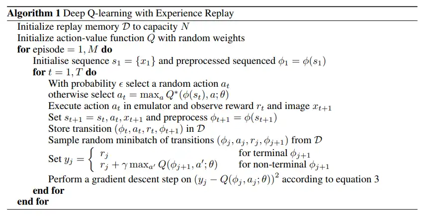
We introduce deep neural networks to do the Q-Learning, hence the name Deep Q-Learning. Instead of calculating Q-values for each state-action pair, we calculate Q-values for all actions given the state and then select the action with maximum q-value. This concept was first introduced in Playing Atari with Deep Reinforcement Learning paper. The authors show that they were able to surpass human experts on three out of seven Atari games tested using deep neural networks to solve these reinforcement problems.

The idea in the paper is that, you capture the Atari screen, use convolutional neural networks to extract the features of the game and then calculate the q-values for each action. Then action with maximum q-value is taken and reward, next state are observed. This data (current state, action taken, reward received, next state) are stored in a fixed sized buffer called replay memory. A batch of random samples with uniform distribution are drawn from this memory and then model is updated. The actions taken by our neural network model are considered as predictions and true actions are calculated using the bellman equation. The error between true value and predictions are calcluated as mean squared error and the model is optimized using this error.

(Source: Playing Atari with Deep Reinfiorcement Learning, Dec 2013)

Let’s try to understand what exactly is happening…

Similar to Q-Learning, we get the state, execute the action using ε-greedy method and observe reward and next state. We then store these observations into a replay memory and use them to update the weights of our neural network which is used to take action. The neural network maps the state to the actions. In next step we sample the observations randomly from the replay memory and the reason we don’t take consecutive observations is that learning is inefficient due to high correlation between the samples. Randomizing the samples break this correlation which helps to reduce the variation of the updates for neural network.

Another reason is that current parameters determine the next data sample that the parameters are trained on. For example, if the maximizing action is to move left then the training samples will be dominated by samples from the left-hand side; if the maximizing action then switches to the right then the training distribution will also switch. This can lead to high divergence in parameters and agent can get stuck in local minima. When randomized samples are used, this behaviour is averaged over many previous states thus smoothing out the learning.

Another confusing thing here is in calculation for values of ground truth. We are using the same network to calculate the y_i and also for prediction. It’s like chasing your own tail. At everytime step we use our neural net to calculate the ground truth for the sampled states and also predict the Q-values for the same, update the network and repeat. So at each timestep we are changing our parameters which means the groud truth also changes. What this means is that everytime the model tries to reach the ground truth of a state, it changes to a new value. Apparently the model works.

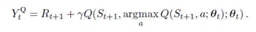
One way to mitigate this problem is by using two neural nets (DQN network and Target network) say with parameters (θ and θ*). Initially we copy the parameters from DQN netwrok to Target network (θ -> θ*), but instead of updating the parameters of target network at each timestep we update them after some fixed time step. By updating the target parameter I mean we copy the new parameter values from DQN network to Targent network after fixed timesteps t. We then use the DQN network for predictions and Target network to calculate the ground truth.

Another solution to above problem is given in Deep Reinforcement learning using Double DQN. The idea is that when we compute the ground truth, we use two networks to decouple the selection from evaluation. So the equation in DQN

changes to

(Notice the θ’).

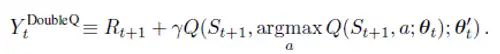
This is done because it was found that when same network is used to select the best action and also for evaluation, the DQN tends to over-estimate values. Hence, we use the DQN network to select best action to take for next state (inner Q-value) argmax Q(S_t+1, a; θ_t) and the Target network to calculate Q(S_t+1, argmax Q(S_t+1, a; θ_t); θ’_t) the ground truth value of taking that action at next state.

Let’s see the DQN in action for Cart and Pole game…

1.Agent at the beginning of training…(Random Actions)

2.Agent after trained for 100 episodes

3.Agent after trained for 200 episodes

Isn’t it amazing!!! Just a few lines of code and our agent can balance a pole on a cart reasonably well. Infact this is not just limited to Cart and Pole Game, you can even train our agent to play some old school Atari games like SpaceInvaders, PingPong, Breakout and many more. But to get good results you need to train it for a long time. Here is the link for the complete code for running DQN for Cart and Pole.

In the next article, we will look at Policy Gradient Methods and solve the same Cart and Pole game to compare the results with Deep Q-Learning.